Tutorial
In the tutorial, we will show you two examples of using ACQDP. The first one is to use the tensor network functionalities to experiment with tensor network states. The second one is to use the circuit library to experiment with the fidelity of GHZ states under various noise models.
MPS State
In this section, we create two random ring-MPS states and calculate their fidelity.
An MPS state is a quantum state formulated as a centipede-shaped tensor network. We first define a random MPS state on a ring, with bond dimension and number of qubits given as the input:
from acqdp.tensor_network import TensorNetwork, normalize
import numpy

def MPS(num_qubits, bond_dim):
    a = TensorNetwork()
    for i in range(num_qubits):
        tensor = numpy.random.normal(size=(2, bond_dim, bond_dim)) +\
                    1j * numpy.random.normal(size=(2, bond_dim, bond_dim))
        a.add_node(i, edges=[(i, 'o'), (i, 'i'), ((i+1) % num_qubits, 'i')], tensor=tensor)
        a.open_edge((i, 'o'))
    return normalize(a)
This constructs an MPS state of the following form, where the internal connections (i, ‘i’) have bond dimension bond_dim and the outgoing wires (i, ‘o’) have bond dimension 2 representing a qubit system.
Note that normalize() computes the frobenius norm of the tensor network, which already involves tensor network contraction.
For a further break down, in the code we first defined a tensor network:
a = TensorNetwork()
Each tensor i is of shape (2, bond_dim, bond_dim). We add the tensor into the tensor network by specifying its connection in the tensor network:
a.add_node(i, edges=[(i, 'o'), (i, 'i'), ((i+1) % num_qubits, 'i')], tensor=tensor)
Finally, the outgoing edges [(i, ‘o’)] needs to be opened:
a.open_edge((i, 'o'))
This allows us to get two random MPS states:
a = MPS(10, 3)
b = MPS(10, 3)
To calculate the fidelity of the two states, we put them into a single tensor network representing their inner product:
c = TensorNetwork()
c.add_node('a', range(10), a)
c.add_node('b', range(10), ~b)
Here, The tensor network c is constructed by adding the two tensor valued objects a and ~b into the tensor network. The outgoing edges of a are identified as 0 to 9 in c, and that matches the outgoing edges of b. As no open edges is indicated in c, it sums over all the indices 0 to 9 and yield the inner product of a and b. (Note that the complex conjugate of b is added instead of b itself.)
This tensor network c takes two tensor valued objects a and b which are not necessarily tensors. This is a feature of the ACQDP: components in tensor networks do not have to be tensors, which allows nested structures of tensor networks to be easily constructed. The fidelity is then the absolute value of the inner product:
print("Fidelity = {}".format(numpy.abs(c.contract()) ** 2))
GHZ State
The next example features our circuit module, which allows simulation of quantum computation supported by the powerful tensor network engine. A priliminary noise model is also included.
A \(n\)-qubit GHZ state, also known as “Schroedinger cat states” or just “cat states”, are defined as \(\frac{1}{\sqrt2}\left(|0\rangle^{\otimes n}+|1\rangle^{\otimes n}\right)\). A \(n\)-qubit GHZ state can be prepared by setting the first qubit \(|+\rangle\), and apply CNOT gate sequentially from the first qubit to all the other qubits. In ACQDP, we first define the circuit preparing the GHZ state:
from acqdp.circuit import Circuit, HGate, CNOTGate, ZeroState

def GHZState(n):
    a = Circuit().append(ZeroState, [0]).append(HGate, [0])
    for i in range(n - 1):
        a.append(ZeroState, [i + 1])
        a.append(CNOTGate, [0, i + 1])
    return a
A GHZ state then can be constructed upon calling \(GHZState(n)\). A 4-qubit GHZ state is then
a = GHZState(4)
a is right now a syntactic representation of the GHZ state as a gate sequence. To examine the state as a tensor representing the pure state vector,
a_tensor = a.tensor_pure
print(a_tensor.contract())
gives the output
array([[[[0.70710678, 0.        ],
        [0.        , 0.        ]],

        [[0.        , 0.        ],
        [0.        , 0.        ]]],


      [[[0.        , 0.        ],
        [0.        , 0.        ]],

        [[0.        , 0.        ],
        [0.        , 0.70710678]]]]).
The tensor_pure of a circuit object returns the tensor network representing it as a pure operation, i.e. a state vector, an isometry, or a projective measurement. In this case we do get the state vector; the density matrix will be returned if we choose to contract the tensor_density.
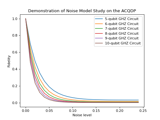
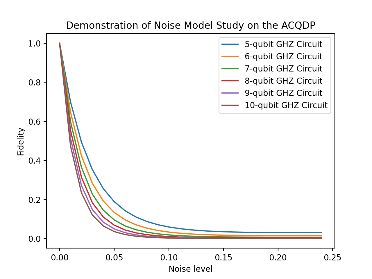
We are now interested in how the fidelity is preserved under simplified noise models.
from acqdp.circuit import add_noise, Depolarization
b = add_noise(a, Depolarization(0.01))
The quantum state b representing noisy preparation of the GHZ state is no longer pure. To compute the fidelity of b and a, we compute the probability of postselecting b on the state a, i.e. concatenate b with ~a:
c = (b | ~a)
print(c.tensor_density.contract())
which gives the result 0.7572548016539656.
The landscape of the fidelity with respect to the depolarization strength is given in the following figure:
(Source code, png, hires.png, pdf)
